January 2026
Target 1: Baseten

SFG
INTRODUCTION
We select the publicly available Orpheus-TTS deployment served via Baseten as a target. The objective is to characterize its performance envelope and exceed it through system-level optimizations as a reference for what organizations and engineers can look to achieve internally or in collaboration with SFG. What follows documents a methodology that can be applied to latency sensitive systems with similar structure, independent of model choice or deployment environment.
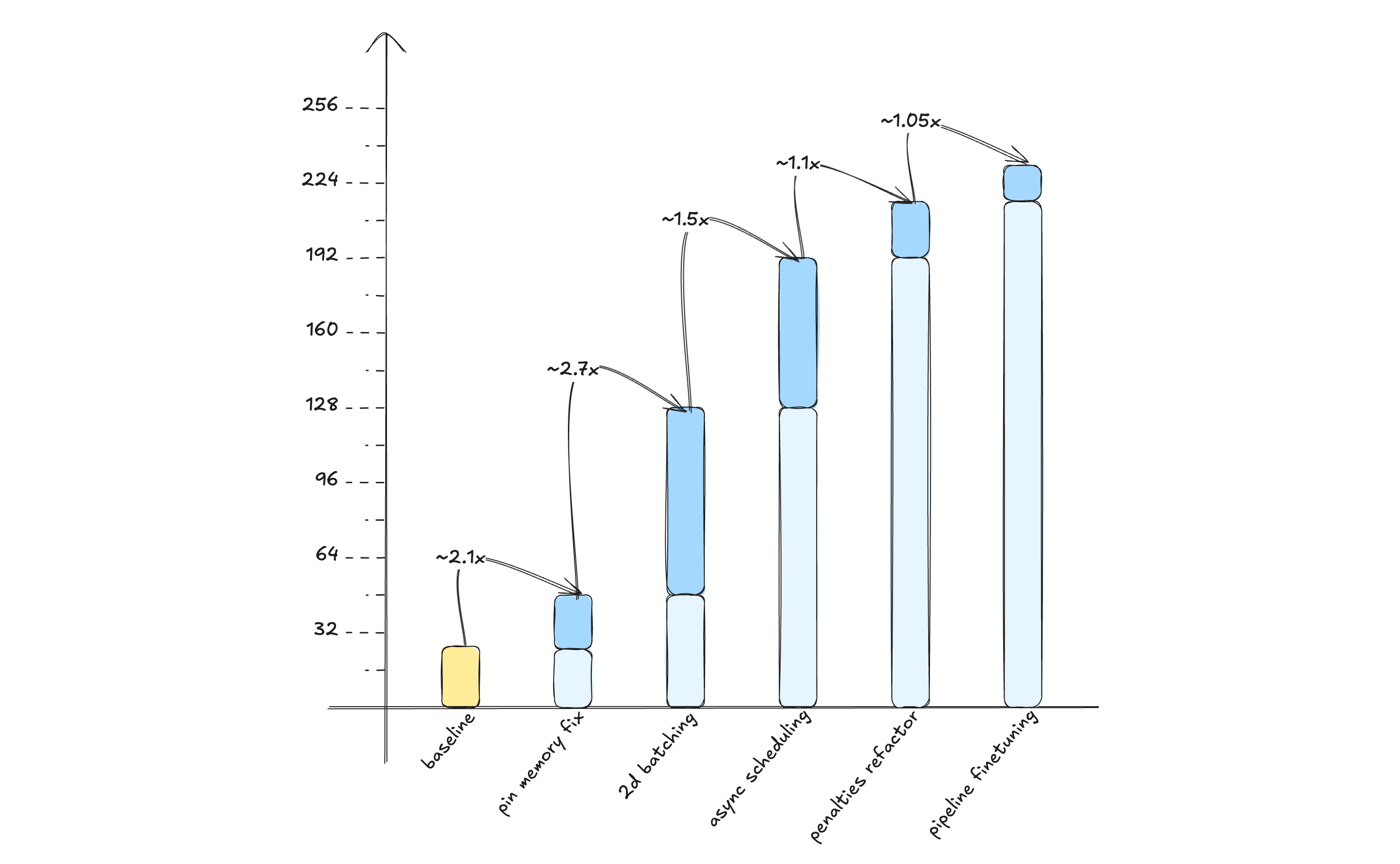
At baseline, the system sustains approximately 24 concurrent real-time connections per H100 GPU while meeting strict p99 latency and real-time factor constraints. After optimization, the same deployment sustains 216 concurrent connections per GPU under identical constraints. This represents a ~10x increase in effective throughput, achieved without modifying model architecture, retraining weights, or relying on specialized hardware.
In a representative production deployment provisioned with 100 H100 GPUs, this baseline corresponds to an average concurrency of 2,400 streams. After optimization, the same aggregate serving capacity can be delivered with approximately 10 GPUs, each sustaining around 240 concurrent connections. As a result, annual accelerator spend drops from roughly $1.4M to $140k while delivering identical service capacity.
TTS Production Deployments
There exists a wide variety of text-to-speech architectures, ranging from fully end-to-end approaches to newer LLM-based designs. This work examines the latter.
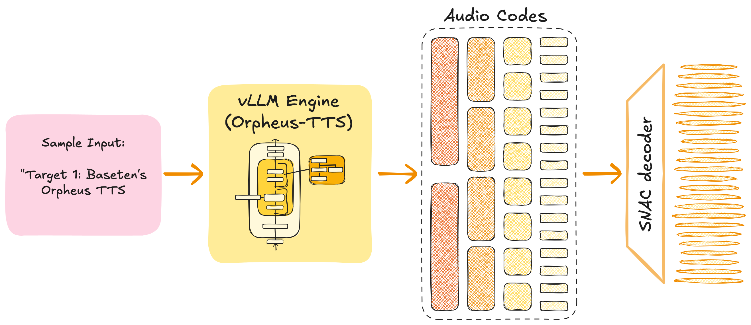
This modern approach, based on an LLM fine-tuned to generate audio features, consists of two main modules. The first and most resource-demanding module is the engine that hosts the LLM, which translates input text into audio features. These features are subsequently decoded into synthesized audio waveforms by the second module, referred to as the codec decoder.
Over the course of this work, we use the Orpheus-TTS open-source model, a fine-tuned variant of LLaMA 3.2 3B developed by Canopy Labs, together with the 19.8 M-parameter SNAC (Multi-Scale Neural Audio Codec) decoder for converting predicted audio tokens back into a waveform. These models are selected as representative, open-source implementations with comparable architecture and scale, ensuring that the system-level optimizations developed here transfer directly to similar deployments.
Eval Configuration
Text-to-speech inference stacks are typically evaluated using Time to First Byte (TTFB) and Real-Time Factor (RTF)1. Unlike more commonly referenced text-based latency measures, these metrics directly capture perceived end-user performance. We also provide our chosen node configuration for the worklog.
- Time to First Byte (TTFB): Measures the elapsed time between a TTS request being issued and the receipt of the first byte of synthesized audio. It captures the combined impact of request handling, acoustic feature generation, feature decoding, and any pre- or post-processing steps between modules. In interactive applications, TTFB is a critical indicator of responsiveness, as it determines how quickly audio playback can begin.
- Real-Time Factor (RTF): Defined as the ratio between the time required to generate audio and the duration of the generated audio. An RTF of 1.0 corresponds to real-time generation, while values below 1.0 indicate faster-than-real-time performance. RTF is particularly important for streaming scenarios, as it ensures audio can be consumed continuously without interruption.
- Node Configuration: All development, profiling, benchmarking, and stress testing were conducted on a node with the configuration detailed below. This setup was intentionally selected as a representative, production-grade inference environment, pairing a high-bandwidth accelerator with a CPU offering sufficient compute and memory to avoid host-side bottlenecks.
- CPU: Intel Xeon Platinum 8481C (26 vCPUs, 234 GB)
- Accelerator: 1× NVIDIA H100 SXM (80 GB @ 3.35 TB/s)2
The H100 SXM platform serves as a stable and widely deployed reference point for high-end inference workloads; the system-level optimizations presented are not hardware-specific and are expected to carry forward to newer accelerator generations.
Optimization Scope
Much of the existing inference optimization literature focuses on model-level techniques, ranging from straightforward methods such as weight quantization or pruning to more complex approaches like speculative decoding or custom attention kernels. These techniques can materially improve per-kernel efficiency and throughput, but they address only a single axis of optimization.
End-to-end inference performance is frequently dominated by system-level effects, including scheduling, resource allocation, CPU–GPU interaction, and pipeline coupling. This work focuses on system-level optimizations that improve behavior across the full inference pipeline by tightening interactions between components, mitigating cross-module bottlenecks, and reducing end-to-end latency under load.
System-level optimizations form a superset that can include model-level techniques while extending to architectural, pipeline-level, and scheduling improvements. These optimizations treat the system holistically rather than isolating individual kernels or modules.
A holistic view of the system exposes performance improvements that remain invisible when the model is treated in isolation. Model-level optimizations are largely orthogonal to the techniques presented here; their effects compound with system-level improvements rather than overlapping. This framing keeps the work applicable across a broad range of models, deployments, and inference pipelines.
This worklog intentionally excludes model-level optimization. Model-centric techniques are well covered in existing literature, while system-level effects are less commonly documented despite their impact on real-world performance. The work that follows documents an empirical, iterative performance engineering process in which bottlenecks are discovered through measurement and resolved incrementally. The emphasis is on method rather than individual optimizations, with the goal of providing a process that generalizes across systems.
Baseline and Baseten
Before initiating any optimization effort, we conduct an internal performance assessment to establish a clear baseline of a system’s current capabilities. This baseline reflects the behavior of a representative, production-grade deployment and serves as the reference point for all subsequent optimization work.
We begin by analyzing how the pipeline behaves under load. At this stage, the focus is intentionally limited to high-level performance metrics and overall system behavior, avoiding low-level profiling tools. This approach allows us to rapidly build intuition about system dynamics under stress and to identify which components warrant deeper investigation. This is particularly valuable in multi-module systems, where the primary bottleneck is often non-obvious. Because collecting these metrics introduces negligible overhead, tracking them is generally recommended even in production environments.
For this initial analysis, we rely on telemetry metrics exposed by the vLLM engine, the primary and most resource-intensive module in the pipeline34.
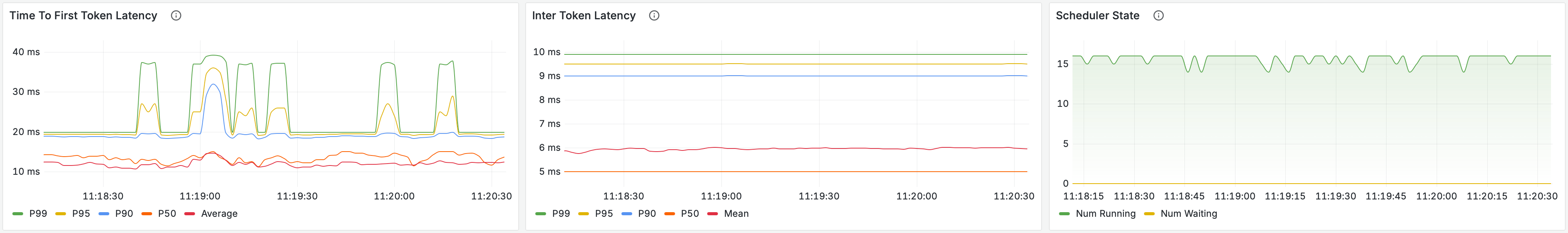
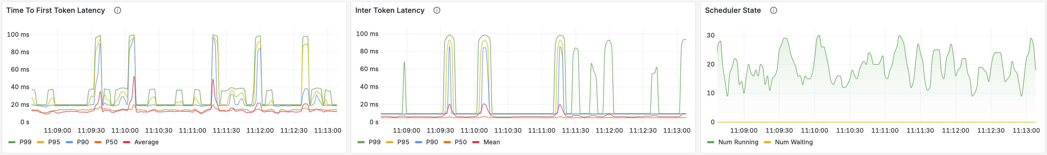
These snapshots already indicate that the system is not operating smoothly under increased load. The first issue to note is the emergence of pronounced ITL spikes at 24 and 32 concurrent connections. At 16 concurrent connections, inter token latency remains stable at approximately 6 ms, with a p99 around 10 ms. These values are expected given the model size and hardware configuration. In contrast, the spikes observed at higher concurrency represent more than a tenfold increase over the steady state average. This behavior is not characteristic of healthy decode execution and indicates intermittent stalls in token generation. Because the system is shared, these stalls could originate from several sources. At this stage, the vLLM engine is the most likely locus and the natural starting point for investigation.
A second signal appears in the scheduler state as concurrency increases. Rather than remaining stable, the number of running and waiting requests begins to oscillate more aggressively at higher load. This pattern suggests that the decoding stage cannot sustain the rate at which acoustic features are produced, introducing back pressure into the pipeline. Although decoding occurs after acoustic feature generation, it participates in the same execution and scheduling pool. When decoding falls behind, active requests are unable to complete and release capacity, which prevents new requests from entering execution. As a result, the engine alternates between brief periods of progress and enforced idle time, effectively capping throughput well below the system’s theoretical capacity.
Baseten’s Orpheus-TTS deployment serves as an external performance reference for this system. Publicly reported results indicate support for up to 24 concurrent connections. We independently evaluated Baseten’s inference service and observed that it could reliably sustain higher load than reported.
In our measurements, Baseten sustained up to 40 concurrent connections per node while continuing to meet p99 TTFB and RTF requirements. This establishes a practical reference point and represents a 1.6× increase over the customer’s original production baseline. The results below report stress test outcomes across all configurations, including this reference5.
| Step @ Concurrency | TTFB (ms) Mean / P90 / P99 | RTF Mean / P90 / P99 | Perf Gain |
|---|---|---|---|
| Baseline @ 16 | 280 / 393 / 475 | 0.477 / 0.489 / 0.520 | NA |
| Baseline @ 24 | 482 / 639 / 1022 | 0.654 / 0.750 / 0.830 | 1.0x |
| Baseline @ 32 | 515 / 746 / 1991 | 0.910 / 1.091 / 1.405 | NA |
| Baseten's FP8 Deployment @ 40 | 418 / 491 / 545 | 0.931 / 0.969 / 0.988 | 1.6x |
The aggregate load test results are consistent with the behavior observed in the telemetry dashboards. As concurrency increases, both RTF and TTFB degrade in ways that materially affect user experience. At 24 concurrent connections, large ITL spikes begin to appear but remain sufficiently rare that the p99 RTF requirement remains below 1, allowing real-time playback to be preserved. At 32 concurrent connections, TTFB degrades more sharply, with p99 values exceeding acceptable thresholds and users waiting up to two seconds for an initial response.
The results also show a growing dispersion in both TTFB and RTF as load increases, reflected in the widening separation between mean, p90, and p99 values. The particularly large gap between p90 and p99 for TTFB indicates that performance degradation is concentrated in a small number of extreme outliers rather than uniformly distributed across requests. This pattern is characteristic of intermittent pipeline stalls rather than sustained throughput saturation.
These observations point to system-level bottlenecks that manifest only under higher concurrency and motivate the optimization steps applied in the following sections, which are model- and architecture-agnostic.
Opt 1: Pinned Memory
Although the baseline analysis pointed toward potential sources of instability, we deliberately deferred any optimization in code until we obtained concrete profiling evidence. Optimizing without clear attribution risks addressing symptoms rather than causes.
Premature optimization is the root of all evil.
Donald Knuth
Given that the baseline behavior suggested intermittent stalls within the engine that emerged only under higher load, we began by profiling the vLLM engine itself. For this initial investigation, we used the PyTorch built-in profiler, which is already integrated into vLLM and is well suited for exploratory analysis across complex execution paths. At this stage, we had only a coarse hypothesis about the source of the issue. Had the problem been isolated to a specific compute kernel, more specialized tools such as NVIDIA Nsight would have been more appropriate.
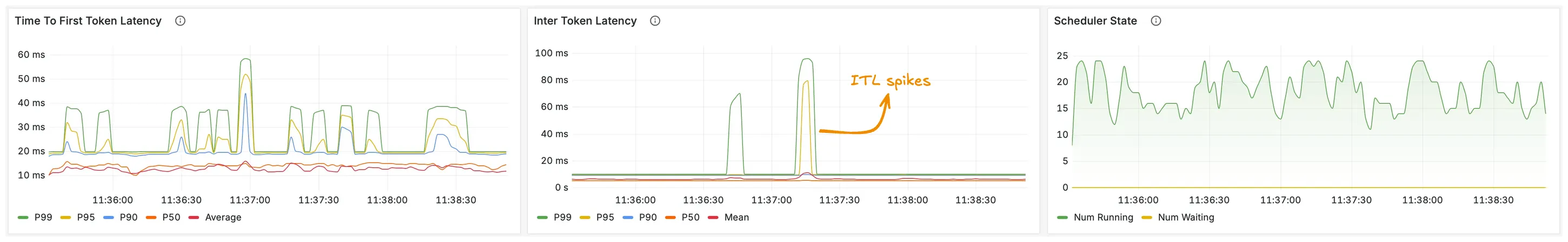
Profiling confirmed the presence of a rare but severe stall affecting the entire engine. Under load, we consistently observed an individual operation taking approximately 70 ms to complete. This event appeared sporadically and was absent from most forward passes, making it difficult to detect without targeted profiling. When it did occur, however, it dominated execution time and aligned closely with the latency spikes observed in the baseline measurements.
The profiler trace below highlights this behavior. An operation that is effectively negligible in the common case occasionally expands to nearly 78 ms, temporarily stalling the engine and contributing directly to the observed tail latency.
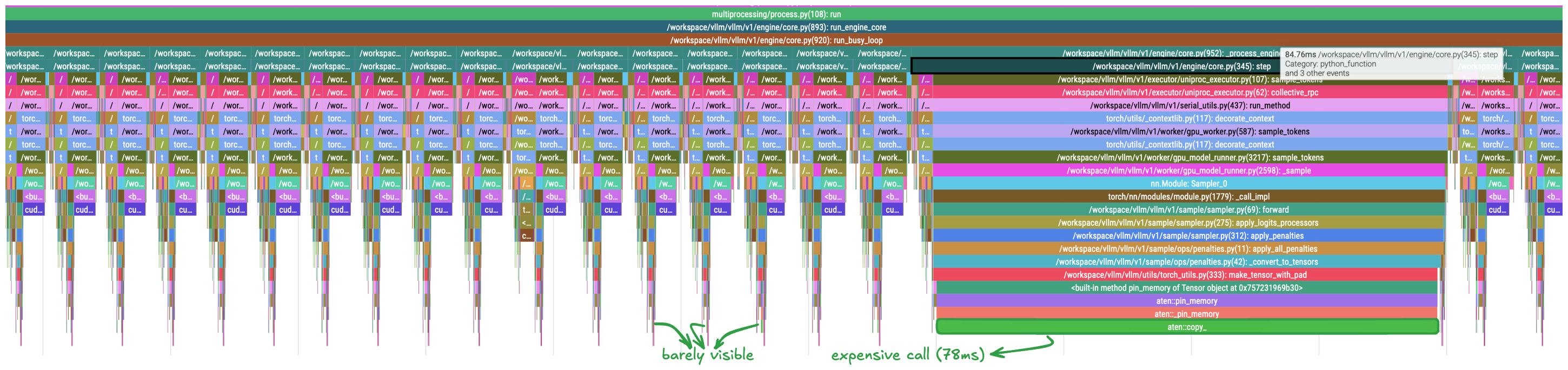
Inspection shows that the long-latency event originates in the sampling stage of the engine step. More specifically, it arises during the application of sampling penalties. Along this path, the engine invokes an auxiliary function,
make_tensor_with_pad, which occasionally expands into a long-running synchronous operation.Two observations are especially useful. The exact call path responsible for the stall is unambiguous, and the operation executes synchronously on the CPU, blocking the main thread. Resolving this event would directly address the ITL spikes observed in the previous section. The dominant cost arises within a call to PyTorch’s
pin_memory operator, which triggers an explicit copy from pageable memory into locked (pinned) memory.Locked memory is a special region of CPU memory that the operating system guarantees will not be paged out to disk. This property makes it directly accessible by the GPU’s Direct Memory Access (DMA) engine, enabling faster data transfers between host and device memory. When data resides in regular pageable memory, the CUDA driver must first copy it into a temporary pinned buffer before initiating the device transfer, introducing additional latency and synchronization overhead. The
pin_memory operator performs this copy explicitly so that the transfer to the device can begin as soon as it is scheduled.Correct use of this operator however is subtle, and the PyTorch team provides explicit guidance on avoiding common performance pitfalls. Reviewing the auxiliary function’s implementation against that guidance makes the issue apparent. Within
make_tensor_with_pad, the code follows a documented anti-pattern.The guide notes that performing an explicit copy from pageable memory into pinned memory, followed by a non-blocking transfer to the device, can be slower than issuing a direct copy to the device. Although both approaches ultimately move data along the same path --> from pageable to pinned memory and then to the device --> managing the copy explicitly on the host introduces additional latency compared to allowing the driver to orchestrate the transfer.
Avoiding this anti-pattern requires a minimal change: removing the explicit pinned-memory copy and delegating the entire transfer pipeline to the driver.
After applying this change, a follow-up profiling session confirms that the issue is resolved. The long-running events disappear entirely, and engine step execution becomes uniform. All steps complete in approximately 8 ms, with no observable stalls.
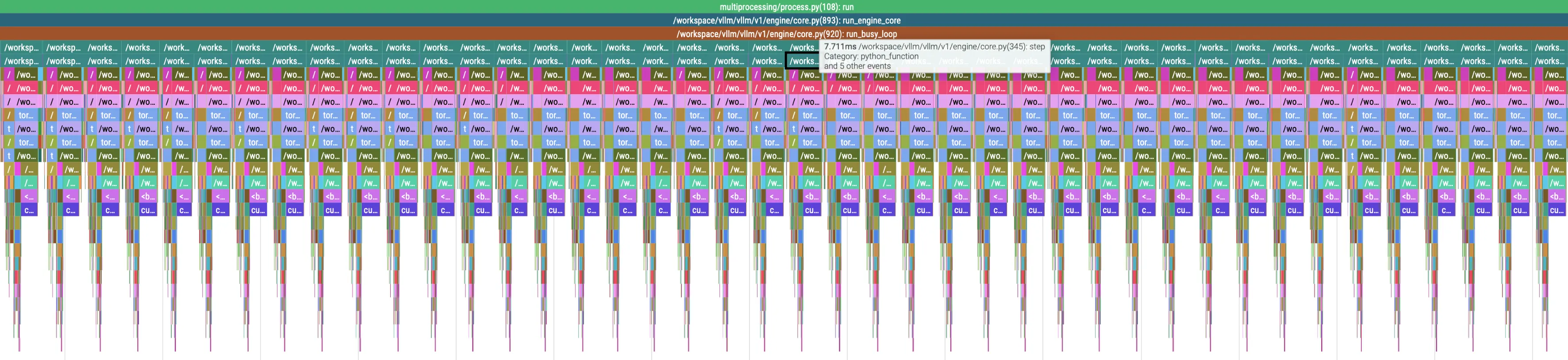
As calls to
pin_memory() followed by non-blocking device transfers are explicitly discouraged in PyTorch’s guidance, we removed the explicit host-side pinning step and allowed the CUDA driver to manage the transfer end-to-end in our evaluation setup.The effect of this change is immediately visible in both the profiler trace and the benchmark results. The long-running synchronous events disappear entirely, and engine step execution becomes uniform. As shown in the trace below, all engine steps now complete in approximately 8 ms, with no sporadic stalls or CPU-side blocking.
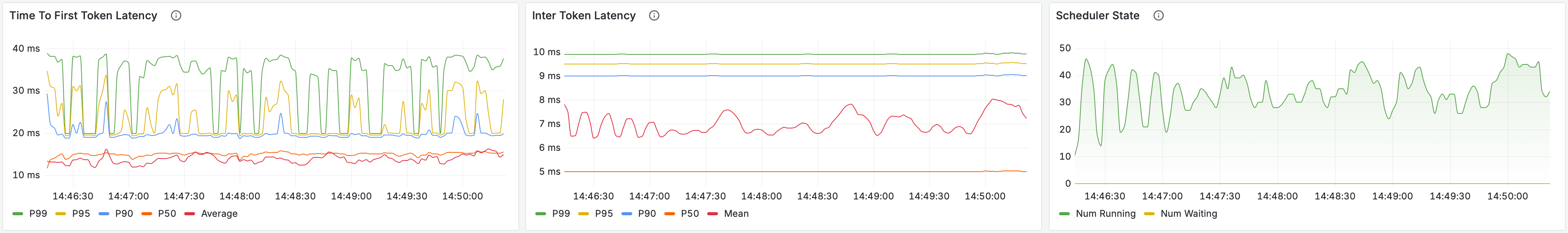
This improvement is also reflected in end-to-end metrics. The system now sustains a concurrency of 48 live connections, more than twice the previous stable level. Inter-token latency becomes uniform and no longer exhibits large spikes, despite the increased load. Crucially, the system continues to satisfy the p99 RTF requirement, confirming that the underlying bottleneck has been resolved and no longer constrains throughput or stability.
| Step @ Concurrency | TTFB (ms) Mean / P90 / P99 | RTF Mean / P90 / P99 | Perf Gain |
|---|---|---|---|
| Baseline @ 16 | 280 / 393 / 475 | 0.477 / 0.489 / 0.520 | NA |
| Baseline @ 24 | 482 / 639 / 1022 | 0.654 / 0.750 / 0.830 | 1.0x |
| Baseline @ 32 | 515 / 746 / 1991 | 0.910 / 1.091 / 1.405 | NA |
| Baseten's FP8 Deployment @ 40 | 418 / 491 / 545 | 0.931 / 0.969 / 0.988 | 1.6x |
| Opt 1: Pin Memory @ 48 | 1091 / 1671 / 2490 | 0.747 / 0.841 / 0.971 | 2.0x |
With the pinned memory fix in place, the system reaches a new steady operating point. Sustained concurrency increases from 24 to 48 live connections per node, while p99 RTF remains below 1 and ITL becomes stable with no observable spikes. Engine step execution time collapses from sporadic outliers of up to ~80 ms to a uniform ~8 ms, confirming that the CPU-side stall identified in the baseline analysis has been eliminated.
At this point, further gains are no longer limited by host-side synchronization but by the rate at which decode work can be amortized across concurrent requests. This shift is visible in the scheduler state, which shows the engine operating below saturation despite increased concurrency. GPU utilization remains suboptimal, and the number of active decoding requests does not fully occupy available compute capacity. In other words, removing the pinned-memory bottleneck exposes decoding efficiency as the next limiting factor in the TTS inference pipeline.
This motivates the next optimization step, which targets decode-side throughput by increasing effective batch utilization under load.
Opt 2: 2D Batching
With the host-side stall removed, the system reaches a new steady operating regime at 48 concurrent connections. At this point, engine execution is stable, ITL remains uniform, and p99 RTF constraints are met. However, scheduler state and GPU utilization indicate that the system is no longer limited by synchronization overhead but by how efficiently decode work is amortized across concurrent requests.
To understand this behavior, we shift from module-level profiling to system-wide analysis. The goal is no longer to isolate a single pathological call, but to identify broader execution patterns that limit decode-side throughput under load. For this phase, we rely on NVIDIA Nsight developer tools, which provide visibility into GPU execution, kernel scheduling, and concurrency patterns that are not accessible through the PyTorch Profiler.
All profiling data presented below was collected while the system sustained 48 concurrent connections. Based on earlier observations, acoustic feature decoding was the primary candidate for the next bottleneck. To make decode behavior explicit in the trace, we annotated the relevant decoding paths using NVTX, allowing us to directly correlate decode activity with GPU utilization and scheduler behavior.
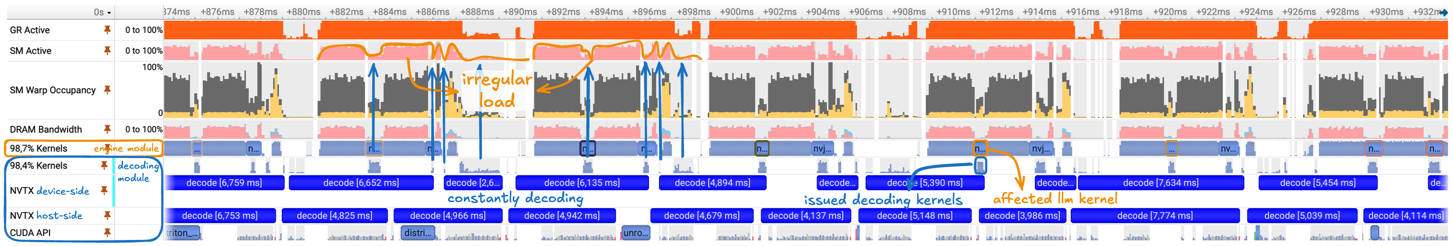
As shown by the NVTX annotations, the system continuously issues decode operations for acoustic features. Each individual decode is relatively small in isolation, as reflected by the short kernel durations visible in the kernel track. However, because these decode operations are interleaved with LLM forward passes, their cumulative impact on execution is significant.
In a steady-state LLM workload without competing GPU activity, forward passes execute smoothly with uniform kernel scheduling. In contrast, under concurrent TTS load, each decode introduces brief but frequent interruptions that fragment GPU execution. This interference is visible as irregular fluctuations in both SM Active and SM Warp Occupancy, indicating that the GPU repeatedly transitions between partially utilized and underutilized states. These transitions align directly with the decode ranges highlighted in the trace.
Although each decode operation is lightweight, issuing them independently prevents effective amortization of kernel launch and scheduling overhead. As concurrency increases, these overheads accumulate, limiting throughput and preventing the GPU from reaching sustained high utilization during the forward pass. The result is inefficient overlap between decoding and LLM execution, even though neither component is individually compute-heavy.
There are several possible approaches to addressing this behavior. One option would be to offload decoding to dedicated hardware, allowing it to execute independently. In this setting, however, decode latency lies on the critical path, and additional device transfers would quickly outweigh any potential benefit.
Another option is to further optimize the decoding kernels themselves. Techniques such as
torch.compile can fuse operations and reduce per-decode overhead. While beneficial, kernel fusion alone does not address the fundamental issue: issuing decode work at fine granularity still incurs repeated launch and synchronization costs that scale with concurrency.The remaining option is to restructure how decode work is scheduled so that overheads are amortized across multiple requests. This motivates the use of dynamic batching at the decode stage, which we describe next.

When a system repeatedly performs small, identical computations over different inputs, batching is the primary mechanism for improving efficiency. By grouping multiple invocations into a single execution, fixed overheads such as scheduling, kernel launch, and synchronization are amortized, while the underlying computation benefits from increased parallelism and denser execution.
In tensor-based architectures, batching is often implemented by aggregating inputs along an additional dimension, allowing the accelerator to execute a larger, more efficient operation. For static workloads, this can be done ahead of time, making batching straightforward and highly effective.
Inference workloads, and real-time systems in particular, complicate this picture. Computations are triggered by independent requests arriving at unpredictable times, and strict latency constraints limit how long the system can wait to form a batch. In many cases, these constraints make batching impractical.
In our setting, however, decode-side batching is both feasible and necessary. As shown in the previous section, issuing decode work for each request independently introduces persistent background interference that fragments GPU execution and limits throughput. By batching decode operations, the system can replace this continuous stream of small invocations with short, well-defined execution windows, reducing overhead and improving overlap with LLM execution.
Because request arrival is inherently bursty and non-uniform, a static batching policy is insufficient. Instead, we employ dynamic batching, in which incoming decode requests are accumulated as they arrive and execution is triggered either when a batch reaches a target size or when a maximum waiting time is exceeded. This approach allows us to trade off throughput gains against latency constraints in a controlled manner and aligns naturally with the real-time requirements of the TTS pipeline. An overview of dynamic batching challenges in deep learning systems is provided in this report.
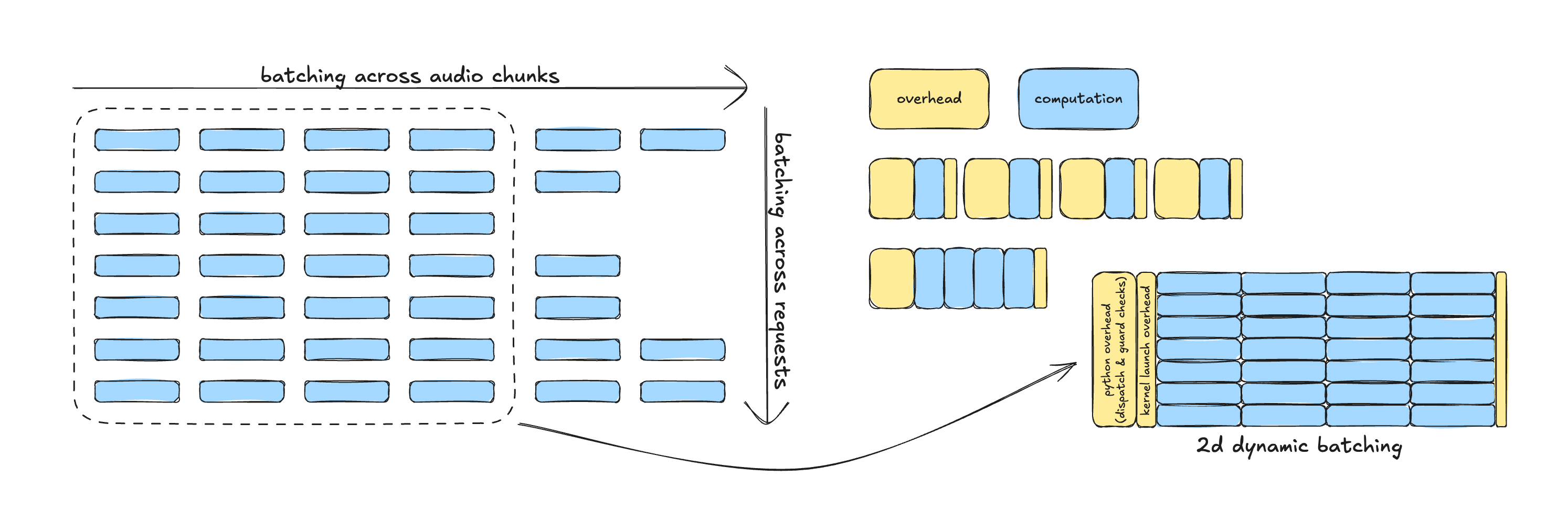
By batching decode work across both audio chunks and concurrent requests, the decoding stage shifts from a continuous stream of fine-grained invocations into a small number of dense execution windows. This restructuring amortizes Python dispatch, scheduling, and kernel launch overhead across substantially more useful computation, reducing interference with the LLM forward pass and improving overall GPU utilization.
In addition to batching, we enabled
torch.compile for the decoding path using default compilation settings and without specialized tuning. Even in isolation, this change is effective: in a non-batched configuration, compiled decoding reduces average execution time by more than 4×, from approximately 4 ms to under 1 ms per decode step. Combined with two-dimensional dynamic batching, decoding is no longer a persistent background workload but a compact, predictable computation that can be efficiently overlapped with LLM execution.The impact of this change is visible in the following profiling trace.
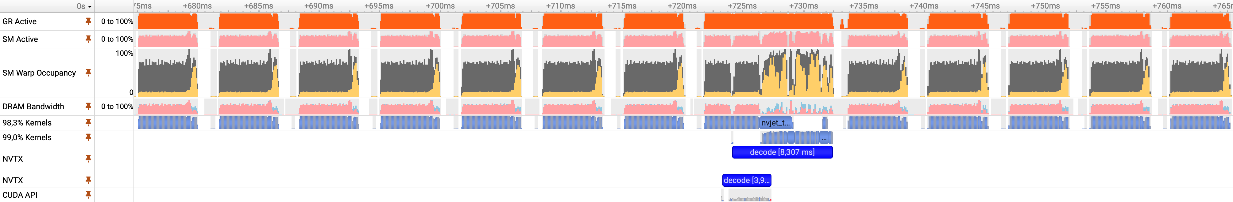
As shown in the updated profiling trace, the decoding module now introduces load only within short, well-defined execution windows, leaving the remainder of the runtime free of decode-related overhead. Each batched decode invocation now takes approximately 8–9 ms to complete. While this is roughly twice the duration of a single unbatched decode, each invocation processes more than 100× as many acoustic features due to two-dimensional batching.
As a result, the effective efficiency of the decoding stage improves by over 50×. Decode execution shifts from a persistent source of fine-grained interference into a compact, high-density workload that can be efficiently amortized and overlapped with LLM computation.
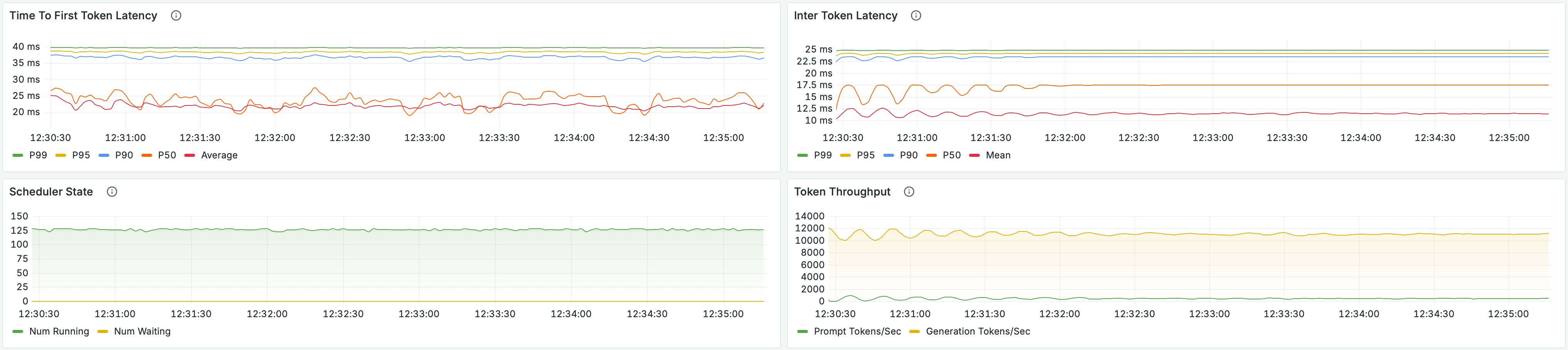
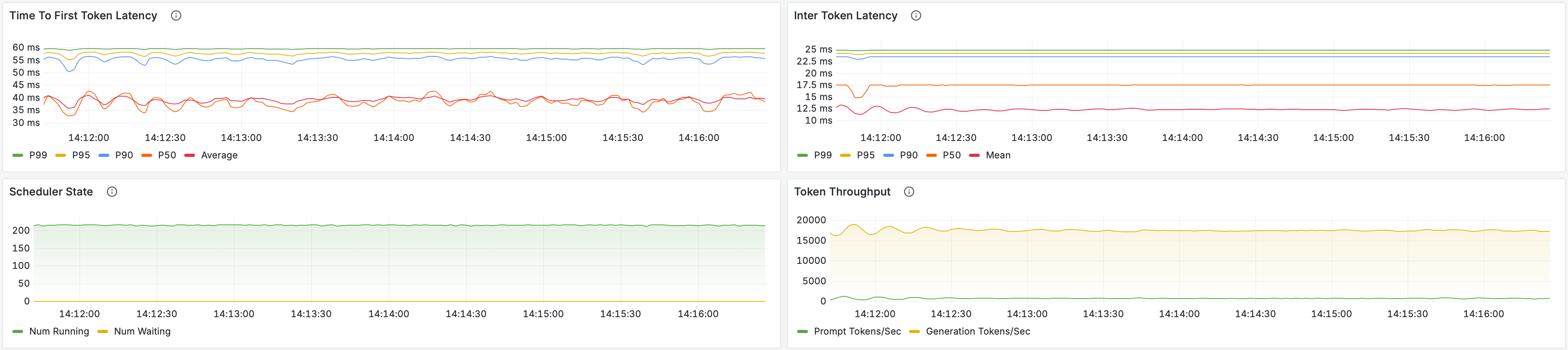
The metrics shown below were collected under a load of 128 concurrent connections, corresponding to approximately 2.7× the load used in the previous evaluation. Under this load, the scheduler state remains stable and uniform, indicating that decoding is able to keep pace with acoustic feature generation. This is a critical change from earlier stages, where scheduler instability was the primary signal of a bottleneck.
The stability of the scheduler under maximum load implies two properties of the system. First, acoustic features are decoded at approximately the same rate at which they are produced. Second, decoding completes almost immediately after feature generation, rather than lagging behind and accumulating backlog. In practice, this means the generation and decoding stages now operate in close synchronization, allowing the pipeline to scale without introducing additional tail latency.
| Step @ Concurrency | TTFB (ms) Mean / P90 / P99 | RTF Mean / P90 / P99 | Perf Gain |
|---|---|---|---|
| Baseline @ 16 | 280 / 393 / 475 | 0.477 / 0.489 / 0.520 | NA |
| Baseline @ 24 | 482 / 639 / 1022 | 0.654 / 0.750 / 0.830 | 1.0x |
| Baseline @ 32 | 515 / 746 / 1991 | 0.910 / 1.091 / 1.405 | NA |
| Baseten's FP8 Deployment @ 40 | 418 / 491 / 545 | 0.931 / 0.969 / 0.988 | 1.6x |
| Opt 1: Pin Memory @ 48 | 1091 / 1671 / 2490 | 0.747 / 0.841 / 0.971 | 2.0x |
| Opt 2: 2D Batching @ 128 | 691 / 736 / 809 | 0.892 / 0.912 / 0.924 | 5.3x |
In addition to improved scheduler stability, these changes produce corresponding gains across user-facing performance metrics. Token throughput now scales smoothly with increasing load, and the TTFB distribution tightens significantly, with no large p99 outliers. Under the previous configuration, p99 TTFB exceeded 2 seconds with a mean near 1 second. After two-dimensional dynamic batching, mean TTFB decreases to approximately 700 ms with a p99 under 800 ms.
Taken together, these results confirm that the decoding stage has transitioned from a dominant, system-wide bottleneck into a non-limiting component with predictable execution characteristics. At a sustained concurrency of 128 connections, corresponding to a 5.3× increase over the baseline reference, the system continues to satisfy p99 RTF requirements while maintaining stable scheduler behavior.
At this stage, decoding is no longer the limiting factor for overall system throughput. This does not imply that decoding is fully optimized, but rather that it has been removed from the critical path. Further improvements can now be pursued incrementally and safely, for example through tighter batching heuristics, stricter latency bounds, or more aggressive compilation strategies. We address one such refinement in the final optimization step.
Opt 3: Async Scheduling
As in earlier stages, we rely on NVIDIA Nsight profiling tools to analyze system behavior. This profiling snapshot was captured while the system was operating at 128 concurrent connections, corresponding to the highest sustained load achieved after the previous optimization step. We intentionally profile the system at its current operating limit, as bottlenecks that materially affect throughput and tail latency often emerge only at scale.
At lower concurrency, these effects can remain hidden or appear insignificant. Conversely, profiling far beyond the system’s stable operating regime can obscure root causes due to overlapping failure modes and burst-induced instability. By profiling at the maximum supported load, we isolate the constraints that directly limit further scaling under realistic operating conditions.
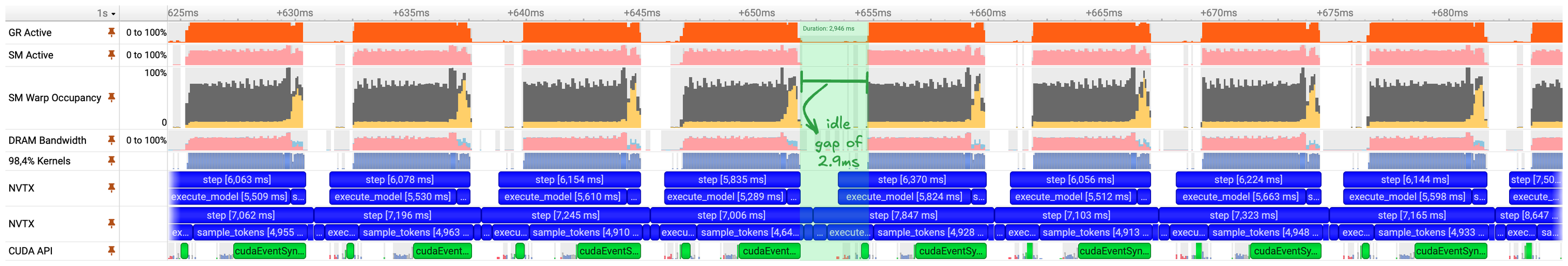
Although the workload appears well structured at first glance, the profiling trace reveals large idle gaps between successive forward passes. During these gaps, GPU utilization drops despite pending work, indicating that the accelerator is frequently stalled waiting on CPU-side scheduling and synchronization.
For large models at low concurrency, such gaps are typically negligible. The computational cost of each forward pass dominates, and CPU-side scheduling and request handling complete quickly by comparison. In contrast, under high concurrency with a relatively small model, these same overheads become first-order effects. Many scheduling, preprocessing, and post-processing steps are inherently sequential and must be performed per request, making them difficult to batch or parallelize.
At sufficient load, these synchronization points accumulate and fragment execution, as shown in the trace. While it may appear that such gaps are unavoidable given the sequential nature of request handling and decoding, this is not entirely the case. A substantial portion of this idle time can be eliminated by overlapping independent work rather than executing it serially.
This motivates the use of asynchronous scheduling, which shifts the execution model away from strict step-level synchronization and toward overlapping computation and coordination wherever possible. Instead of stalling the accelerator at each synchronization boundary, independent tasks are allowed to progress concurrently, minimizing idle time and improving overall utilization.

The idle gaps visible in the trace are primarily consumed by scheduling and output processing. In the synchronous execution model, the system waits for a forward pass to complete before scheduling the next batch of work, and output processing similarly waits for sampling to finish before consuming results. These dependencies introduce synchronization barriers in both directions, leaving the accelerator idle between steps.
While these gaps appear small in absolute terms, they are significant relative to the execution time of the forward pass for this model, which ranges from approximately 6 to 10 ms depending on load composition. Even a 2 ms idle period represents a substantial fraction of useful compute time. Under sustained load, these gaps accumulate, reducing throughput, increasing latency, and leaving expensive accelerator resources underutilized.
There is no fundamental requirement for these operations to be blocking. Scheduling and output processing can be overlapped with model execution so that the host continues preparing future work while the accelerator is busy. This shifts the execution model from strict step-level synchronization to overlapping computation wherever possible. As described by Woosuk, “the primary goal is to minimize scheduler overhead by overlapping scheduling with model execution, making the scheduler operate one step ahead of the current execution.”
Support for asynchronous scheduling in vLLM was first introduced in #19970 and has been under active development as of #27679. While this mode was not initially enabled by default due to compatibility constraints with other optimizations, it is sufficiently mature and stable for our workload. Enabling asynchronous scheduling allows scheduling and output processing to progress concurrently with model execution, substantially reducing idle time between steps.
Before examining the results, it is important to acknowledge the limits of this approach. Completely eliminating idle gaps is impractical given the inherently sequential aspects of transformer decoding and the irregular, input-dependent nature of inference workloads. Some host–device synchronization is unavoidable, particularly for control flow and result handling. However, by overlapping these operations wherever possible, their impact can be reduced to a marginal contribution to overall latency. The following profiling results illustrate the effect of this change.
Update: asynchronous scheduling is now enabled by default in vLLM via #27614.
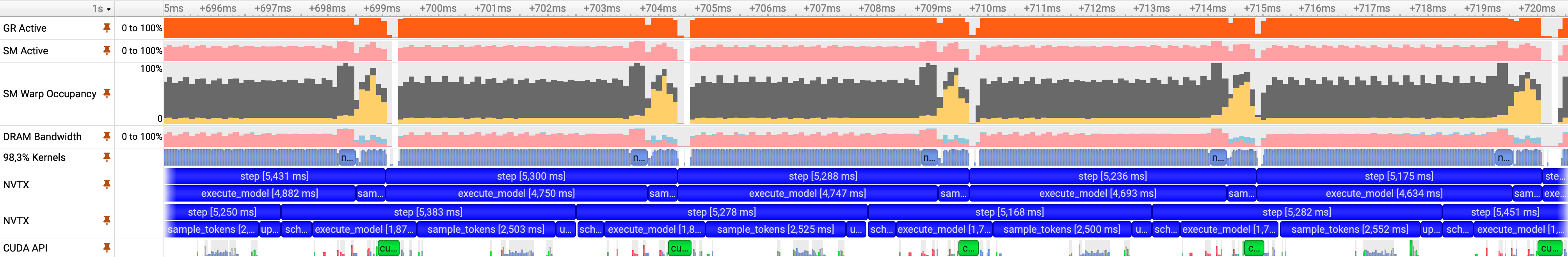
As shown in the updated profiling trace, the idle gaps between successive forward passes are substantially reduced. GPU utilization is now nearly continuous, with only a small synchronization barrier on the order of a few hundred microseconds per step. Prior to enabling asynchronous scheduling, the step duration averaged 7.8 ms with a standard deviation of 1.6 ms. After the change, the average step duration decreases to 6.1 ms, with a standard deviation of 1.9 ms, corresponding to a 1.27× speedup at the step level.
This reduction in idle time translates directly into improved throughput and latency, as well as higher effective utilization of the accelerator.
We next evaluate the system under a sustained load of 192 concurrent connections, which we determined to be the maximum concurrency that can be maintained while keeping RTF < 1. This represents a 1.5× increase over the previous maximum sustained load of 128 connections.
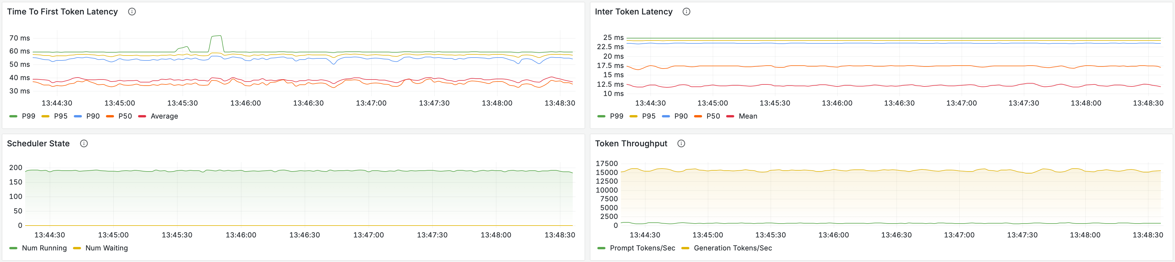
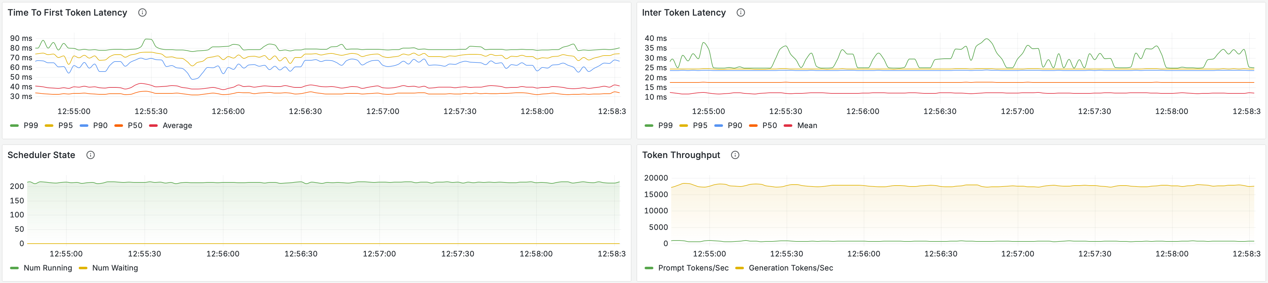
The updated Grafana metrics and summary table show that scheduler state remains stable under this load, token throughput scales smoothly, and both TTFB and inter-token latency remain well behaved. In aggregate, asynchronous scheduling increases supported concurrency from 128 to 192, corresponding to an 8.0× improvement over the original baseline reference.
| Step @ Concurrency | TTFB (ms) Mean / P90 / P99 | RTF Mean / P90 / P99 | Perf Gain |
|---|---|---|---|
| Baseline @ 16 | 280 / 393 / 475 | 0.477 / 0.489 / 0.520 | NA |
| Baseline @ 24 | 482 / 639 / 1022 | 0.654 / 0.750 / 0.830 | 1.0x |
| Baseline @ 32 | 515 / 746 / 1991 | 0.910 / 1.091 / 1.405 | NA |
| Baseten's FP8 Deployment @ 40 | 418 / 491 / 545 | 0.931 / 0.969 / 0.988 | 1.6x |
| Opt 1: Pin Memory @ 48 | 1091 / 1671 / 2490 | 0.747 / 0.841 / 0.971 | 2.0x |
| Opt 2: 2D Batching @ 128 | 691 / 736 / 809 | 0.892 / 0.912 / 0.924 | 5.3x |
| Opt 3: Async Scheduling @ 192 | 944 / 1025 / 1263 | 0.931 / 0.958 / 0.980 | 8.0x |
The updated Grafana metrics and summary table show that scheduler state remains stable under this load, token throughput scales smoothly, and both TTFB and inter-token latency remain well behaved. In aggregate, asynchronous scheduling increases supported concurrency from 128 to 192, corresponding to an 8.0× improvement over the original baseline reference.
Taken together, these results demonstrate that asynchronous scheduling effectively removes scheduler-induced idle time as a limiting factor. By overlapping scheduling and output processing with model execution, the system approaches saturation without introducing instability or violating real-time constraints.
While asynchronous scheduling was still considered experimental at the time of this work, we validated its correctness through extensive end-to-end testing under production-representative workloads. This gave us sufficient confidence to deploy it for our use case, despite it not being enabled by default in vLLM at the time. (As of recent releases, asynchronous scheduling is now enabled by default.)
Opt 4: Penalty Refactors
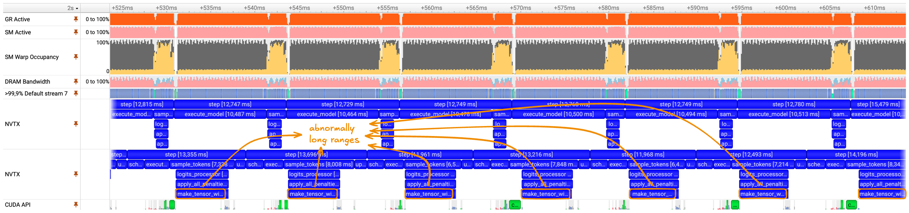
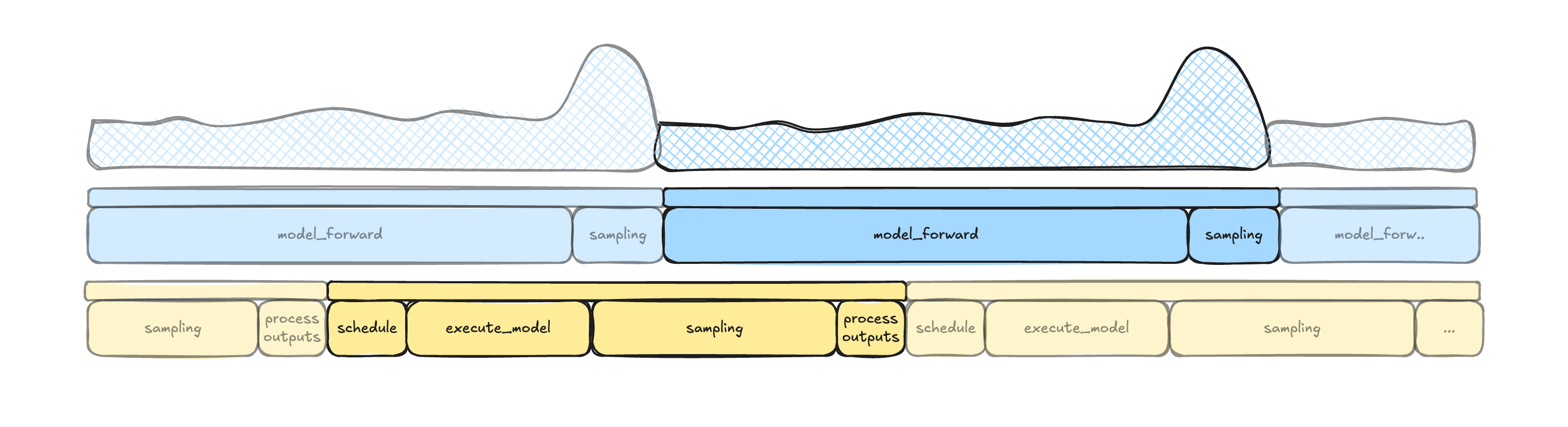
Profiling at high concurrency reveals that sampling remains unusually expensive, particularly the portion executed synchronously on the host. This behavior is visible in the NVTX trace, where several long ranges appear on the CPU timeline with no corresponding activity on the device.
The two NVTX tracks represent the same logical code paths observed from different perspectives. The upper track shows ranges as observed on the accelerator, while the lower track shows those same ranges as observed on the host. Not all host ranges have a one-to-one correspondence with device execution. Ranges that do not issue GPU work appear only on the host, indicating CPU-only execution. Additionally, even when both host and device ranges exist, their timings do not align exactly due to host–device dependencies and stream scheduling. Device work cannot begin until it is enqueued by the host, and queued operations execute only when the stream becomes available. As a result, host ranges may complete before the corresponding device ranges begin, particularly for non-blocking operations.
Among all annotated ranges, one stands out clearly:
make_tensor_with_pad. This range is both long and entirely host-bound, with no associated device activity. Its execution time dominates the sampling phase and directly contributes to scheduler stalls and idle gaps observed earlier in the pipeline. A zoomed-in view highlights this behavior more clearly.This observation indicates that the sampling penalty logic is not limited by GPU execution but by CPU-side tensor preparation and synchronization. Because this work executes synchronously on the host, it blocks the scheduling of subsequent steps and propagates latency through the pipeline.
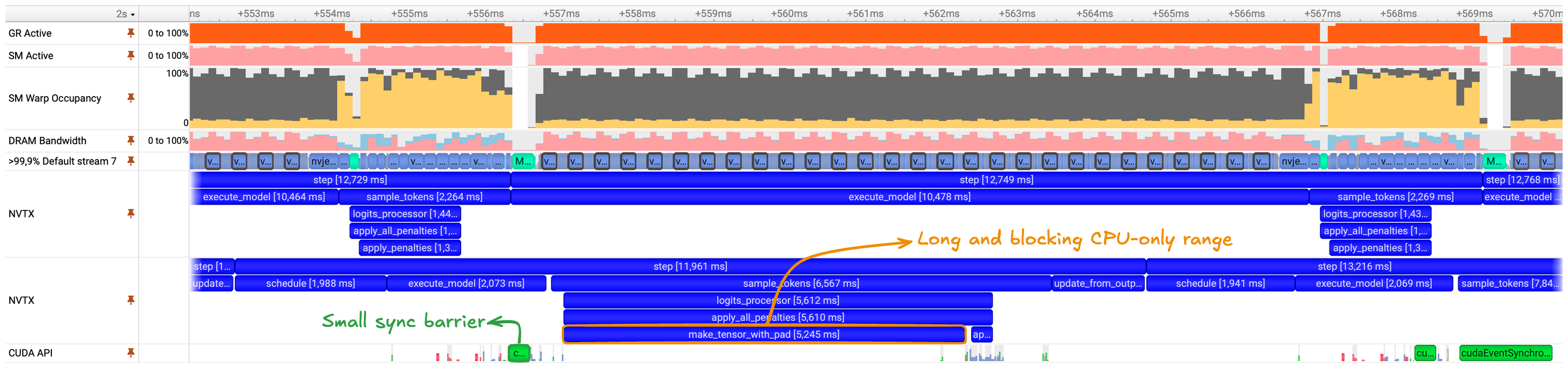
The highlighted range corresponds to a CPU-only operation in the sampling path responsible for converting output tokens from a list-based representation into a dense tensor. This operation executes synchronously on the host and introduces a blocking point before subsequent model execution can proceed.
Inspection of the code path shows that the cost does not originate from the auxiliary function itself, but from how output tokens are tracked upstream. While the vLLM engine allocates static tensors to track requests, generated tokens, and associated metadata, penalty computation relies on a separate representation in the form of a list of lists of integers. As a result,
make_tensor_with_pad is invoked on every forward step to materialize a dense tensor required for downstream computation.Given this input representation, the conversion is unavoidable and inherently expensive. It involves repeated, sequential memory copies across multiple locations and cannot be made efficient in isolation. This indicates that the bottleneck should not be addressed at the level of the auxiliary function, but earlier in the pipeline.
To eliminate this overhead, we refactored the data structure used to track output tokens entirely. The revised approach mirrors how the engine tracks other sequences, relying on preallocated tensors that are incrementally updated rather than constructing new tensor instances at each step. This removes the need for repeated list-to-tensor conversions during penalty computation.
To ensure compatibility with asynchronous scheduling, this refactor required explicit updates to the output state so that the cumulative tensor representation remained consistent and up to date. Importantly, this was done without introducing additional synchronization barriers. The necessary bookkeeping was incorporated into an existing synchronization point, preserving the asynchronous execution model.
This change was integrated as an independent plugin. The solution remains suitable for upstream integration and will be linked once the corresponding pull request is available.
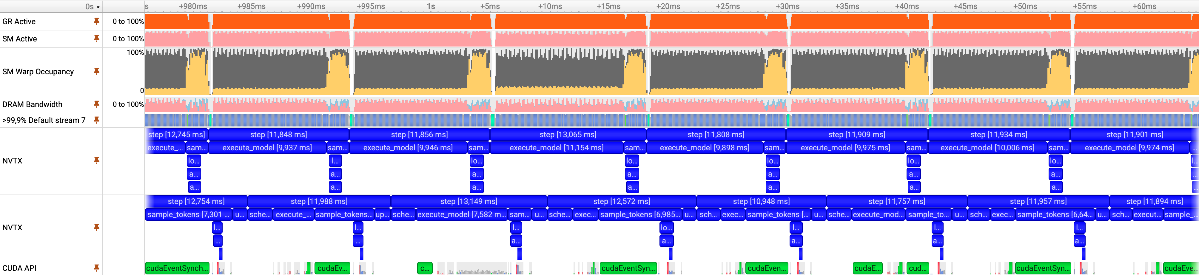
The load test results are consistent with the behavior observed in profiling. Refactoring the penalties path removes the final host-side stall in the sampling stage and enables a further increase in sustained concurrency from 192 to 216 live connections while continuing to satisfy the real-time constraint (RTF < 1). This corresponds to a 9.0× increase over the original baseline.
In addition to higher supported concurrency, token throughput increases from approximately 15k tokens/s to nearly 17k tokens/s, while the TTFB distribution continues to improve. Mean TTFB decreases further, and p99 latency remains tightly bounded, indicating that the additional throughput is achieved without introducing new tail latency.
With this change, sampling penalties no longer introduce blocking CPU-side work on the critical path. Combined with asynchronous scheduling and two-dimensional dynamic batching, the pipeline now sustains higher load with predictable latency and stable scheduler behavior.
| Step @ Concurrency | TTFB (ms) Mean / P90 / P99 | RTF Mean / P90 / P99 | Perf Gain |
|---|---|---|---|
| Baseline @ 16 | 280 / 393 / 475 | 0.477 / 0.489 / 0.520 | NA |
| Baseline @ 24 | 482 / 639 / 1022 | 0.654 / 0.750 / 0.830 | 1.0x |
| Baseline @ 32 | 515 / 746 / 1991 | 0.910 / 1.091 / 1.405 | NA |
| Baseten's FP8 Deployment @ 40 | 418 / 491 / 545 | 0.931 / 0.969 / 0.988 | 1.6x |
| Opt 1: Pin Memory @ 48 | 1091 / 1671 / 2490 | 0.747 / 0.841 / 0.971 | 2.0x |
| Opt 2: 2D Batching @ 128 | 691 / 736 / 809 | 0.892 / 0.912 / 0.924 | 5.3x |
| Opt 3: Async Scheduling @ 192 | 944 / 1025 / 1263 | 0.931 / 0.958 / 0.980 | 8.0x |
| Opt 4: Penalty Refactors @ 128 | 908 / 1010 / 1089 | 0.929 / 0.953 / 0.965 | 9.0x |
At this point, all major bottlenecks identified during profiling have been addressed, and further gains move into the regime of incremental refinement.
Opt 5: Pipeline Tuning
With the dominant structural bottlenecks removed, residual inefficiencies become the limiting factor. At this stage, no single component disproportionately constrains performance. Instead, throughput and latency are governed by the cumulative effect of smaller overheads distributed across the pipeline. This final optimization phase focuses on tuning these interactions to meet specific operational targets under sustained load.
Rather than uncovering new bottlenecks, this phase consists of targeted parameter adjustments informed by profiling and validated through repeated benchmarking. Each change was evaluated independently to ensure that improvements translated into measurable gains under production-representative conditions. The most impactful adjustments are summarized below:
- More aggressive batching via timeout tuning. The batch timeout was increased by a factor of 3–4 without negatively impacting per-request latency. Because acoustic feature generation already dominates early execution, this additional wait time was effectively free. As a result, decode batches were formed approximately every 0.4 seconds, significantly improving batch density and amortizing overhead more effectively.
- Rebalancing
torch.compileconfigurations between batched and tail paths. Initial compilation settings prioritized reducing overhead for batched decoding, while leaving individual tail requests on the default compilation path due to shape variability. Further analysis showed that tail requests occur more frequently and therefore benefit more from reduced overhead. The configuration was inverted, enabling full CUDA graph capture for tail decoding while relaxing constraints for batched paths. - Reducing compilation overhead through shape padding. To limit the explosion of compiled graphs caused by shape variability, kernel inputs were padded to fixed sizes that are multiples of 8, 16, or 24. This reduced the number of required compiled graphs by up to 24×. As a secondary effect, the effective batch size could be increased from 64 to 256 sequences, matching the engine’s maximum supported capacity.
- Optimizing CPU-to-GPU transfers in batched decoding. The data transfer pipeline was restructured so that CPU-to-GPU copies occur after batching rather than before. Instead of issuing up to 256 small transfers, the system now performs a single large copy per batch. This significantly reduces transfer overhead and improves decode efficiency.
- Eliminating unnecessary I/O in WAV header generation. WAV header construction previously required creating a temporary file, introducing avoidable I/O latency. Replacing this with a direct, in-memory header generation path removed this overhead entirely, reducing TTFB from hundreds of milliseconds to the time required to decode audio tokens alone.
| Step @ Concurrency | TTFB (ms) Mean / P90 / P99 | RTF Mean / P90 / P99 | Perf Gain |
|---|---|---|---|
| Baseline @ 16 | 280 / 393 / 475 | 0.477 / 0.489 / 0.520 | NA |
| Baseline @ 24 | 482 / 639 / 1022 | 0.654 / 0.750 / 0.830 | 1.0x |
| Baseline @ 32 | 515 / 746 / 1991 | 0.910 / 1.091 / 1.405 | NA |
| Baseten's FP8 Deployment @ 40 | 418 / 491 / 545 | 0.931 / 0.969 / 0.988 | 1.6x |
| Opt 1: Pin Memory @ 48 | 1091 / 1671 / 2490 | 0.747 / 0.841 / 0.971 | 2.0x |
| Opt 2: 2D Batching @ 128 | 691 / 736 / 809 | 0.892 / 0.912 / 0.924 | 5.3x |
| Opt 3: Async Scheduling @ 192 | 944 / 1025 / 1263 | 0.931 / 0.958 / 0.980 | 8.0x |
| Opt 4: Penalties Refactor @ 128 | 908 / 1010 / 1089 | 0.929 / 0.953 / 0.965 | 9.0x |
| Opt 5: Pipeline Finetuning @ 216 | 540 / 572 / 630 | 0.963 / 0.985 / 0.992 | 9.0x |
| Opt 5A: FT for TTFB (fp8) @ 200 | 378 / 422 / 453 | 0.821 / 0.839 / 0.861 | 8.3x |
| Opt 5B: FT for RTF (fp8) @ 300 | 2159 / 2724 / 3204 | 0.941 / 0.982 / 0.997 | 12.5x |
The updated stress-test results show that pipeline fine-tuning delivers meaningful gains even after the major structural bottlenecks have been addressed. Through targeted adjustments to batching parameters and compilation modes, TTFB is reduced by nearly 2x while maintaining the same level of concurrency and continuing to satisfy RTF < 1. The highlighted configuration represents a fully optimized system under the original operational constraints.
At this point, further system-level optimizations yield diminishing returns. GPU utilization is high, scheduler behavior is stable, and remaining overheads contribute marginally to end-to-end latency. Additional improvements at the pipeline level would require disproportionate effort relative to their impact.
Beyond this point, further gains come primarily from model-level changes. To illustrate this, the final entries in the table report performance under fp8 quantization, evaluated under two different operating targets. When optimizing for reduced TTFB, the system sustains 200 concurrent connections while maintaining RTF < 0.9 and TTFB < 0.5 s. When optimizing for throughput under looser TTFB constraints, the system scales to 300 concurrent connections while continuing to meet the real-time factor requirement.
These results demonstrate that the optimized pipeline is not only stable under fixed constraints, but also flexible across different latency–throughput trade-offs. While model-level optimizations often compound effectively with system-level improvements, they can also significantly alter resource requirements. In such cases, additional pipeline retuning may be necessary. Speculative decoding is one example of this regime, as introducing an auxiliary model changes compute balance and scheduling dynamics. We leave a detailed treatment of these extensions to future work.
Takeaways
This work documents an iterative performance engineering effort that transformed an LLM-based TTS inference system from supporting 24 concurrent connections per node to sustaining 216 concurrent connections on the same hardware. This represents a 9x increase in per-node serving capacity and translates directly into more than an 80% reduction in serving costs. Relative to previously reported results for Orpheus-TTS deployments, the optimized system exceeds prior state of the art by over 5× while continuing to meet strict real-time constraints.
The optimizations described here did not rely on novel models or specialized hardware. Instead, they emerged from systematically identifying and removing end-to-end bottlenecks across the pipeline, from host–device interaction and scheduling to batching strategy and data structure design. While each individual change was modest in isolation, their compounded effect was substantial.
Several recurring observations from this work generalize beyond this specific system:
- Coupling matters. The degree of coupling between components strongly influences how performance improvements compound. In tightly coupled systems, a bottleneck in one module can suppress utilization elsewhere. Removing that bottleneck often unlocks latent capacity across the pipeline, producing gains that exceed the local improvement itself.
- Iterative optimization is essential. Complex systems rarely expose a single, static bottleneck. Changes frequently alter execution dynamics in unexpected ways, especially under load. Introducing one change at a time, validating its impact, and re-profiling at the new operating point is critical for isolating cause and effect.
- Tooling must match the question. Effective performance work requires choosing the right level of abstraction at each stage. High-level telemetry can surface systemic issues, while low-level traces are often necessary to pinpoint root causes. Mismatches between tooling and the problem being investigated can easily obscure the true source of inefficiency.
- Simplicity is the greatest sophistication. This is a recurring pattern in performance engineering. The difficulty lies not in implementing the fix, but in correctly identifying the bottleneck within a complex, noisy system. In practice, the engineering effort is often dominated by disciplined measurement and careful reasoning, with the final code change being the smallest part of the work.
While this write-up focuses on system-level optimizations, model-level techniques can further extend these results. Such techniques often compound effectively with pipeline improvements, but may also shift resource balance enough to warrant additional system retuning. Exploring these interactions remains an important area for future work.
Limitations
While this work illustrates a general methodology for performance engineering, the specific optimizations described are shaped by the system, workload, and constraints under consideration. The pipeline was tuned against a clearly defined operating envelope, including fixed hardware, latency targets, and load characteristics. As a result, not all configuration choices or trade-offs will transfer directly to environments with different architectures or requirements.
One important limitation is the load profile used for benchmarking and profiling. The system was evaluated under a deliberately constructed load pattern designed to closely reflect the partner’s production workload. Several optimizations, particularly around batching behavior and scheduling, were tuned to perform optimally under that distribution. Improving performance under this specific load required accepting trade-offs, such as favoring lower tail latency over maximizing absolute concurrency. Different request length distributions or traffic patterns may surface different bottlenecks and shift where the true limits lie.
Another constraint is hardware specificity. All experiments were conducted on a fixed hardware configuration, reflecting the deployment environment available at the time. While most of the system-level optimizations discussed here are expected to transfer across accelerators, certain behaviors are hardware- and driver-dependent. For example, the pinned memory issue described earlier manifested only under specific environments. Model-level performance characteristics also vary substantially across hardware platforms. NVIDIA’s Hopper architecture provides extensive support for optimized attention kernels and low-precision execution, which may not be available or as mature on alternative accelerators.
Throughout this work, strict thresholds for real-time factor (RTF) and time to first byte (TTFB) were treated as hard constraints. These requirements narrowed the search space and dictated which avenues were viable to pursue. If these constraints change, for example in offline or asynchronous batch processing settings, the optimization landscape changes as well, and previously unattractive paths may become dominant.
While the concrete fixes presented here are specific, the broader lesson is methodological. Meaningful performance gains emerged not from applying predefined techniques, but from repeatedly instrumenting the system, following the evidence under realistic load, and isolating the factor that most constrained progress at each stage. In complex systems, the hardest part is rarely the fix itself, but recognizing where to look next and knowing when a bottleneck has truly been exhausted.
Further Work
This work intentionally focuses on system-level optimizations, leaving model-level techniques as a clear extension. These approaches introduce a separate set of trade-offs and are best explored incrementally, starting with techniques that are straightforward to prototype and benchmark, such as quantization or pruning. While these methods can introduce quality or accuracy considerations, they are often relatively simple to evaluate in isolation.
A particularly high-potential direction is speculative decoding. Although speculative decoding is often framed as a latency optimization for LLM inference, it spans both training and system design and therefore differs from typical model-only techniques. Implementing speculative decoding generally involves multiple stages, including training a draft model, integrating the drafting phase into the inference pipeline, and verifying outputs against the target model. vLLM already supports several speculative decoding variants and draft-model configurations, making this direction accessible from a systems integration standpoint.
For training draft models, the EAGLE paper series (EAGLE-1, EAGLE-3) provides extensive guidance on training methodology. EAGLE demonstrates that training on extracted hidden states from existing datasets can achieve speedup ratios and acceptance rates comparable to training directly on target-model outputs. In standard text-generation settings, this observation significantly reduces the cost of preparing training data.
The setting considered here differs in an important way. The target model emits acoustic features represented by custom tokens that do not appear in standard text datasets. As a result, the output distribution differs substantially from typical LLM token distributions. In this context, generating a matched dataset by producing acoustic feature targets from representative text samples, and then extracting hidden states from those outputs, is likely necessary to achieve reliable draft-model behavior.
An additional consideration specific to text-to-speech systems is that acoustic features tend to vary smoothly across neighboring steps. Adjacent audio codes often decode to perceptually similar sounds, whereas adjacent text tokens can correspond to entirely different character sequences. This local continuity is highlighted in recent work, which proposes a tolerance-based sampling threshold that explicitly accounts for such structure. Combining this tolerance mechanism with EAGLE-style speculative decoding may offer a promising optimization path for TTS workloads.
Overhead remains a critical factor in evaluating these techniques. In this system, the target model is relatively small and already executes efficiently, which places a tighter latency budget on speculative decoding than in large-model settings. Any gains must outweigh the additional cost of drafting and verification. If the overhead of speculative execution approaches the cost of the original forward pass, speculative decoding can underperform despite being conceptually attractive. Careful measurement and end-to-end evaluation are therefore required before integrating such techniques into latency-sensitive pipelines.
Founder's Remark
A significant amount of performance remains unclaimed, particularly among companies whose valuations are not reflected in their execution.
Happy hunting.